
New Developments in Autonomous Underwater Vehicles
Written by Paul Stankiewicz & Marin Kobilarov, Johns Hopkins University
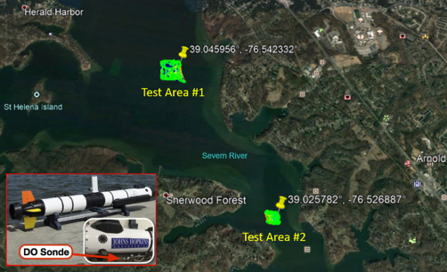
Figure 1: Map of the test areas used for adaptive sampling. All deployments were conducted with an Iver3 AUV pictured in the bottom left.
This past year saw significant progress on developing autonomous underwater vehicle (AUV) technology for use in Chesapeake Bay environmental sampling. AUVs have the capability to adapt their trajectories based on in-situ data to focus sampling efforts on higher-level goals such as mapping environmental phenomena. Giving an AUV these higher-level goals lets the system execute this objective with greater efficiency due to the ability to adapt in response to measurements collected during the mission. In this way, much more information can be gathered about the measurement of interest than is currently available through static buoys or pre-planned trajectories. With regards to monitoring the health of the Chesapeake Bay, these systems allow precise hypoxic volume estimation by augmenting static buoys and ship-based sampling with multiple autonomous vehicles.
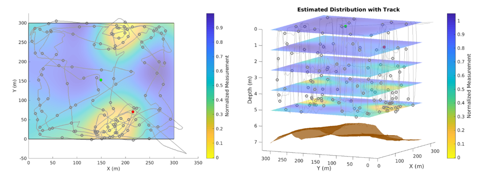
Figure 2: Results of the estimated environmental distribution and vehicle trajectory for test area #1 using a simulated measurement field.
This methodology for data collection was tested over the past year with improved algorithms to perform fully autonomous 3D adaptive sampling operations. These improvements were tested over two deployments in the Severn River, shown in Figure 1. Test area #1 consisted of a 300×300 meter grid with a simulated measurement field of two regions of interest located near the seabed. Test area #2 consisted of a 175×175 meter grid where previously collected measurements were used to create a true dissolved oxygen distribution. Results of the deployments are shown in Figures 2 & 3, where the AUV was able to locate the regions of interest (yellow) in both test areas and preferentially focus its resources on collecting data in these regions. Future work is looking to scale these results to larger areas with longer deployments using a team of underwater and aerial vehicles.
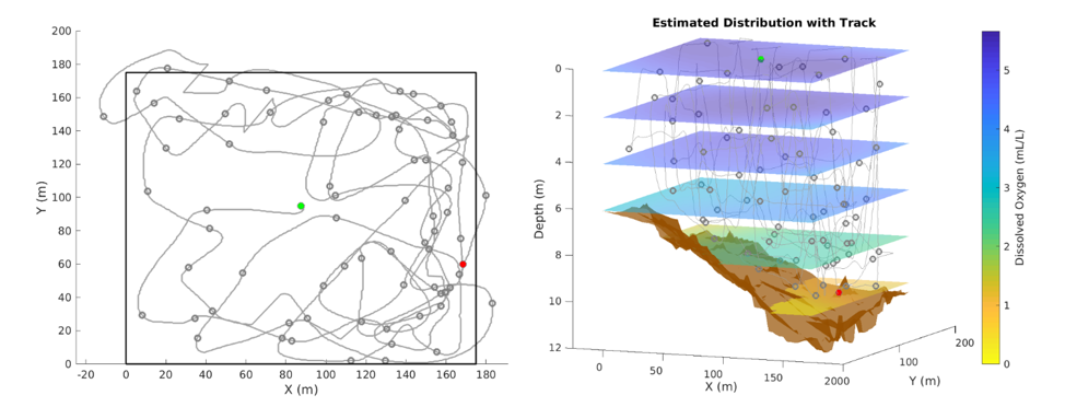
Figure 3: Results of the estimated environmental distribution and vehicle trajectory for test area #2 using dissolved oxygen data.